
How Correlated Positions Silently Multiply Your Risk
A trader who risks one percent per trade on five simultaneous positions does not have one percent risk.

The standard framework for position sizing — risk a fixed percentage of capital per trade — is built on an assumption that is almost never stated explicitly and almost never true in practice. The assumption is that each trade’s outcome is independent of every other trade’s outcome. If that assumption holds, the math works cleanly: five positions at one percent each produce one percent losses when any individual trade stops out, five percent when all five stop out simultaneously, and the probability of the latter is the product of the individual stop probabilities.
When the assumption breaks down — when positions move together because they are driven by the same underlying factor — the math changes entirely. Five correlated positions at one percent each can produce five percent losses not just when all five are wrong, but whenever the shared underlying factor moves against them. The individual position limits mean nothing if the positions themselves are not independent. The risk model looks precise on paper and is systematically misleading in practice.
This newsletter is about what correlation actually means for a trading portfolio, how to measure it in terms that are actionable rather than academic, why it becomes most dangerous precisely when the trader feels most confident, and what structural approaches to position construction prevent correlated risk from accumulating silently until a single market event forces it to reveal itself all at once.
[Download the full printable PDF below.]
WHAT CORRELATION ACTUALLY MEANS FOR A PORTFOLIO
Correlation, in the statistical sense, measures the degree to which two instruments move together. A correlation of positive one means they move in perfect lockstep. A correlation of zero means their movements are completely independent. A correlation of negative one means they move in exactly opposite directions. In practice, most correlated positions in a trading portfolio sit somewhere between zero and positive one, and the precise value matters less than understanding what the correlation implies for how the portfolio behaves under stress.
The practical implication of high positive correlation is that correlated positions tend to lose at the same time. When the underlying factor that drives both positions moves against them, both stop out within the same session or the same few sessions. This means the effective risk of running both simultaneously is not the sum of their individual risks discounted by some diversification benefit — it is much closer to the full combined risk. A portfolio running three highly correlated one-percent positions is not running three independent bets. It is running something closer to one three-percent bet with some timing noise around it.
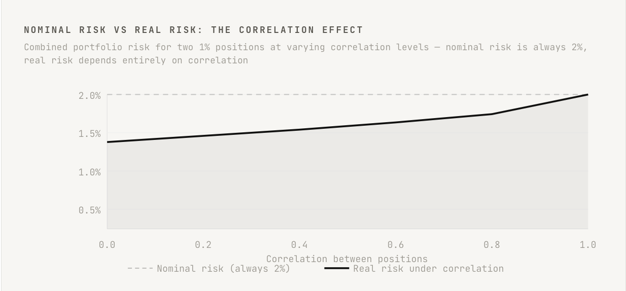
The more insidious version of this problem is partial correlation — positions that are not identical in their drivers but share a meaningful common factor. Two technology stocks in different sectors will not move in perfect lockstep, but during a broad risk-off event they will both sell off. Two momentum positions in different currency pairs will both lose during a sudden reversal in risk appetite. The partial correlation is invisible during normal conditions because the positions move somewhat independently day to day. It becomes fully visible during precisely the periods when the trader least wants to discover it: the high-volatility, high-stress episodes where capital preservation matters most and the account can least afford a simultaneous multi-position drawdown.
PRACTICAL APPLICATION
Before adding any new position to an existing book, answer this question explicitly: what is the primary factor that would cause this position to stop out? Then ask the same question of every position currently open. If two or more positions share the same primary stop-out factor — a broad market move, a dollar index shift, a sector rotation, a change in volatility regime — they are correlated for risk purposes regardless of how different the instruments appear on the surface. This qualitative correlation check takes thirty seconds and catches the most dangerous form of correlation before it enters the portfolio.
THE HIDDEN FACTOR: WHY POSITIONS CORRELATE MORE THAN THEY APPEAR TO
The most common reason traders underestimate the correlation between their positions is that they evaluate correlation at the instrument level rather than the factor level. Two instruments can look completely different — one is a US equity, one is a commodity futures contract — while sharing a dominant common factor that determines their behavior during stress. Both may be highly sensitive to the direction of the US dollar, or to global risk appetite, or to the Fed’s interest rate trajectory. Under normal conditions the idiosyncratic behavior of each instrument dominates and the common factor is invisible. Under stress the common factor dominates and the idiosyncratic behavior disappears.
This factor-level correlation is the form that causes the most damage precisely because it is the most invisible during the period when it is accumulating. A trader building a diversified book of seemingly unrelated positions is often building a concentrated bet on a single macro factor without realizing it. The positions look different. The underlying exposure is not. When the macro factor moves sharply — as it tends to do during the episodes that define calendar-year performance — the apparent diversification provides no protection because it was never genuine diversification to begin with.
Liquidity stress amplifies this effect. During normal sessions, correlated positions may show only moderate co-movement because the mechanisms that link them operate slowly. During a sharp risk-off event, liquidity providers withdraw, bid-ask spreads widen, and the fastest route to reducing exposure is to sell whatever is most liquid rather than whatever is most appropriately sized. This forced liquidation behavior causes previously uncorrelated instruments to move together simply because the same marginal sellers are exiting all of them simultaneously. The stress-period correlation of a portfolio is almost always meaningfully higher than the calm-period correlation, which means the period when the portfolio most needs the protection of diversification is the period when that protection is least available.
“Correlation is low when you do not need it to be low and high when you need it to be low. This is not a coincidence. It is a feature of how markets work under stress.”
PRACTICAL APPLICATION
Map each position in your current book to its two or three dominant macro factors — broad market direction, dollar strength, volatility regime, rate expectations, sector momentum. Do this on a simple grid with positions as rows and factors as columns, marking which factors each position is sensitive to. Any factor column that has more than one mark represents a correlated exposure. The number of marks in that column, multiplied by the individual position risk, approximates the true risk of that factor moving against you. Most traders who complete this exercise for the first time find that their apparent portfolio diversification reduces to two or three concentrated macro bets.
MEASURING WHAT YOU ACTUALLY HAVE: FROM NOMINAL RISK TO REAL RISK
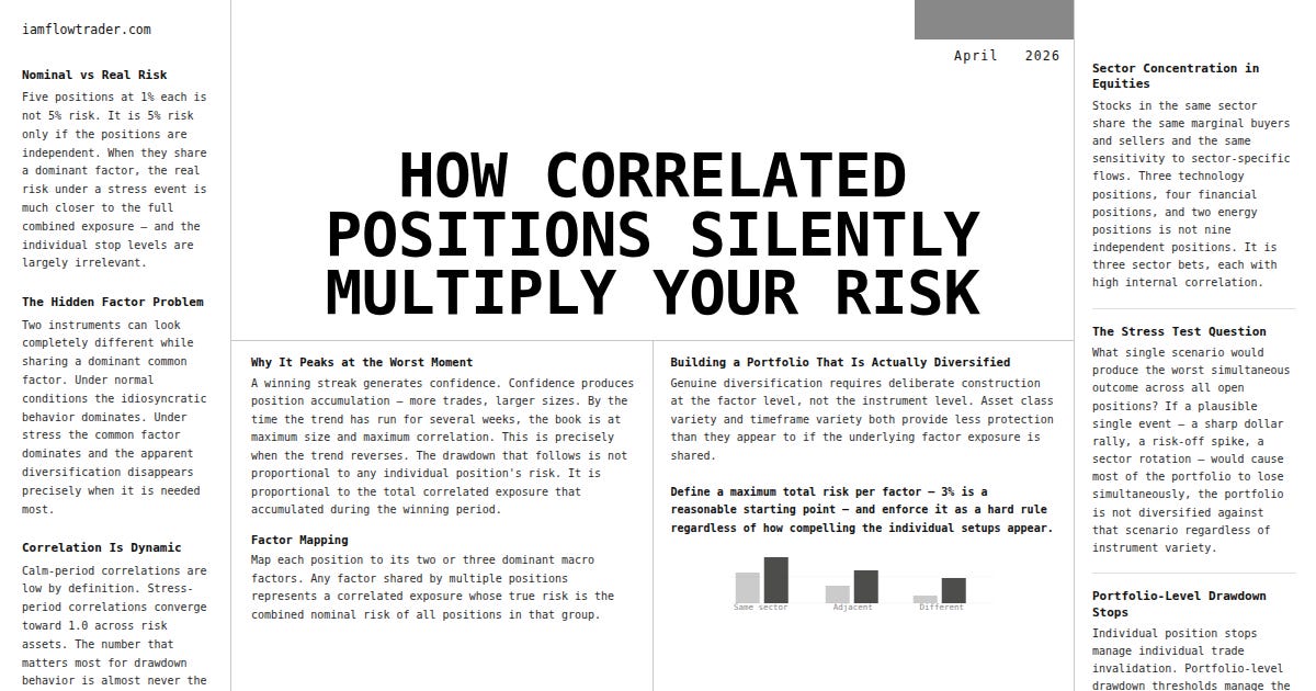
The gap between nominal risk and real risk is the central practical problem that correlation creates. Nominal risk is what the position sizing spreadsheet shows: three positions at one percent each equals three percent total risk. Real risk is what the portfolio actually loses if a correlated stress event occurs: something much closer to three percent in a single session, rather than one percent losses spread across three independent events over an extended period.
The practical framework for converting nominal risk to a more realistic estimate of real risk under correlation requires only two inputs: the individual position sizes and a rough estimate of the pairwise correlation between each pair of positions. For a two-position portfolio, the combined variance under correlation is approximately the sum of individual variances plus two times the correlation times the product of the individual standard deviations. For a practical trading context, this means that two positions each risking one percent with a correlation of 0.8 produce a combined risk profile much closer to two percent than to the square root of two percent that true independence would imply.
A simpler heuristic that captures the same intuition without the formula: group your open positions by their dominant factor, and treat all positions sharing a dominant factor as a single position whose size is their combined nominal risk. If three momentum trades share the same broad market direction as their primary driver, treat them as a single three-percent position for risk management purposes. This simple grouping converts the misleading nominal risk picture into something that more accurately represents the portfolio’s actual exposure to any single adverse event.
PRACTICAL APPLICATION
At the end of each session before adding new positions the following day, group all open positions by dominant factor and sum the nominal risk within each group. If any single factor group exceeds your maximum single-trade risk by more than fifty percent — for example, if you cap individual trades at one percent but a factor group totals two percent — reduce one or more positions in that group before the next session opens. This single rule, applied consistently, prevents the silent accumulation of correlated risk that most traders only discover when a stress event forces the correlation to reveal itself.
WHY CORRELATION RISK PEAKS AT THE WORST POSSIBLE MOMENT
There is a specific sequence of events that makes correlated risk most dangerous, and it follows the same pattern reliably enough to be described almost as a rule. The sequence begins with a period of trending, low-volatility conditions in which a momentum-following or trend-based strategy generates consistent winners. Each winner increases confidence. Each increase in confidence tends to produce a slight expansion of position size or a relaxation of selectivity — more positions taken, larger sizes, or both. By the time the trend has been running for several weeks, the trader’s book is at its most extended: maximum positions, maximum sizes, maximum correlation because every position is a bet on the continuation of the same underlying trend.
This is precisely when the trend reverses. The reversal, when it comes after an extended trending period, tends to be sharp because positioning has become one-sided. The trader who has been building correlated exposure through a winning period now faces the worst possible outcome from that correlation: all positions move against them simultaneously, at maximum size, with no time to reduce exposure gracefully because the move is happening faster than position management can respond. The drawdown that results is not proportional to any individual position’s risk. It is proportional to the total correlated exposure that was allowed to accumulate during the winning period.
The psychological dimension of this dynamic makes it self-reinforcing. A winning streak generates confidence, and confidence suppresses the risk awareness that would otherwise prevent position accumulation. The trader feels in control precisely when the structural risk of the book is at its highest. The feeling of control is a lagging indicator of the preceding performance, not a leading indicator of the portfolio’s resilience to the next adverse event. By the time the event arrives and reveals the true risk, the conditions that created it have been generating good results for long enough that the trader has stopped questioning them.
PRACTICAL APPLICATION
Track your portfolio’s factor concentration alongside your equity curve. After any winning streak of five or more trades, conduct an explicit correlation audit before taking the next new position. List every open position, identify its dominant factor, and calculate the total nominal risk grouped by factor. If the audit reveals that more than sixty percent of total open risk is concentrated in a single factor, reduce to below fifty percent before adding new exposure. Implement this as a standing rule rather than a judgment call, because the judgment call will almost always favor adding the position — confidence is highest precisely when concentration risk is most dangerous.
SECTOR AND INSTRUMENT CORRELATION IN EQUITY TRADING
For equity traders, the most common and most underestimated form of correlation is sector co-movement. Stocks within the same sector share not just business characteristics but also the same marginal buyers and sellers, the same institutional flow dynamics, and the same sensitivity to sector-specific news and macro factors. During a sector rotation — a shift in institutional preference from one sector to another — stocks within the same sector will move together regardless of their individual fundamentals or technical setups. A trader running three technology positions, four financial positions, and two energy positions does not have nine independent positions. They have three sector bets, and the internal correlation within each sector is high enough that the individual position sizing is largely irrelevant to the sector-level risk.
The beta-adjusted correlation is the relevant measure for equity portfolios. A high-beta stock and a low-beta stock in the same sector will not move in perfect lockstep on a daily basis, but during a broad market decline both will sell off, the high-beta name more severely. The correlation of their drawdowns during stress periods is substantially higher than their day-to-day correlation suggests. A portfolio construction approach that uses only day-to-day price correlation to assess diversification will systematically underestimate the stress-period correlation that determines actual drawdown behavior.
Index inclusion creates another invisible correlation. Stocks within the same major index — particularly heavily-weighted components — are subject to passive flows that move them together regardless of individual characteristics. When index funds experience net outflows, they sell across the entire index. When they experience inflows, they buy across the entire index. A trader who is long multiple S&P 500 components is exposed to this passive flow correlation in addition to the fundamental correlations that their factor analysis might capture. The passive flow correlation has grown significantly over the past decade and now represents a meaningful portion of the co-movement in large-cap equity portfolios.
PRACTICAL APPLICATION
Set a hard limit on the number of positions from the same sector you will hold simultaneously, regardless of how compelling each individual setup appears. For most discretionary traders, one to two positions per sector is the appropriate maximum. For positions in adjacent sectors — technology and communications, financials and real estate — apply a combined limit rather than separate limits for each. Track your sector exposure on a simple daily table alongside your position log. Any session where more than forty percent of open positions share a sector or adjacent-sector classification warrants a review of sizing before the next session.
CORRELATION ACROSS ASSET CLASSES AND TIMEFRAMES
Traders who operate across multiple asset classes or multiple timeframes often believe that this variety provides meaningful diversification. It does, but substantially less than it appears to, and the degree to which it fails depends on the same underlying mechanism: shared factor exposure. A trader who is long equities, long crude oil, and long high-yield credit is running three different instruments across three different asset classes. They are also running three expressions of the same underlying view: that risk appetite is expanding and the global growth outlook is favorable. When that view is correct, all three positions profit. When it reverses, all three lose. The asset class diversification is real at the instrument level and largely irrelevant at the factor level.
Timeframe diversification creates a similar illusion. A trader who holds a long-term position in one direction while running short-term trades in the same direction on a lower timeframe is not running two independent strategies. They are running two expressions of the same directional view at different holding periods. If the view is wrong, the short-term trades stop out and then the long-term position also reverses as the directional move continues against them. The timeframe separation provides some protection against whipsaw on the shorter timeframe, but it does not protect against the kind of sustained trend reversal that would invalidate the view across both timeframes simultaneously.
The clearest test of whether apparent diversification is genuine is to ask what single event would cause the maximum simultaneous loss across the portfolio. If there is a plausible single scenario — a sharp move in a specific macro factor, a sudden shift in market regime, a specific geopolitical development — that would cause most or all of the portfolio to lose simultaneously, the portfolio is not genuinely diversified against that scenario regardless of how different the individual positions appear.
+0.6
Approximate correlation between major risk assets during stress periods, regardless of their calm-period correlation. The number that matters most is almost never the one you measured last month.
PRACTICAL APPLICATION
Once per week, run a simple stress test on your current portfolio. Identify the one macro scenario that would produce the worst simultaneous outcome across all open positions — a sharp dollar rally, a sudden risk-off event, a spike in volatility, a sector-specific shock. Estimate what the combined loss would be across the portfolio under that scenario, accounting for the correlation that would likely exist during that specific event. If the stress-scenario loss exceeds three times your average single-trade risk, the portfolio has more concentrated correlated exposure than your individual position limits suggest. Reduce until the stress-scenario loss is within acceptable bounds.
BUILDING A PORTFOLIO THAT IS ACTUALLY DIVERSIFIED
Genuine diversification — the kind that provides actual protection during stress rather than the appearance of protection during calm — requires deliberate construction at the factor level rather than the instrument level. The process begins with a clear map of the factors the strategy is sensitive to, and a conscious decision about which factors the portfolio will concentrate in and which it will limit exposure to.
For a trader running a directional equity strategy, the relevant factors typically include broad market direction, sector momentum, volatility regime, and dollar strength. Genuine diversification means having some positions that benefit from risk-on conditions and some that benefit from risk-off conditions, or alternatively, having all positions on one side of the risk spectrum but limiting the total exposure to that single factor. The first approach — genuine factor diversification — is structurally more robust but harder to implement when a strong trend is running. The second approach — single-factor concentration with hard size limits — is easier to implement and still meaningfully better than unlimited correlated accumulation.
The practical reality is that most directional traders will naturally concentrate in the direction of the prevailing trend, because that is where their setups appear and where their edge operates. This is not a flaw — it is how trend-following and momentum-based strategies work. The risk management response to this reality is not to force artificial diversification across uncorrelated factors that the strategy is not designed to trade. It is to set a hard limit on total factor exposure, maintain that limit regardless of how compelling the setups in the prevailing direction appear, and treat the limit as a non-negotiable constraint rather than a guideline subject to situational override.
PRACTICAL APPLICATION
Define a maximum total risk allocation per factor and enforce it as a hard rule. A reasonable starting point for most discretionary traders is a maximum of three percent total nominal risk in any single factor, regardless of how many individual positions contribute to that factor exposure. If a new setup would push factor exposure above three percent, the existing exposure must be reduced before the new position is added. Write this rule into your trading plan and treat violations as process failures rather than acceptable situational judgments. The judgment will almost always favor taking the trade. The rule is there precisely because the judgment is unreliable at the moment it matters most.
CORRELATION AS A DYNAMIC VARIABLE: MANAGING IT IN REAL TIME
Correlation between positions is not fixed. It changes with market conditions, with volatility levels, and with the distance from a potential stress event. A portfolio that had genuinely diversified factor exposure last week may have concentrated correlated exposure this week if a macro development has changed the correlations between the instruments the trader is holding. Managing correlated risk effectively requires treating correlation as a variable to be monitored rather than a property to be assessed once at the time of position entry and then ignored.
The most reliable leading indicator of correlation compression — the process by which previously uncorrelated positions begin moving together — is a sustained increase in realized volatility across multiple instruments simultaneously. When different instruments in a portfolio all begin showing larger daily ranges at the same time, it is usually because a common macro factor has become the dominant driver across all of them. This is the early signal that calm-period correlations are breaking down and stress-period correlations are emerging. The appropriate response is to reduce total exposure across the board rather than to manage each position individually against its own technical levels.
Position management during stress requires a different framework than position management during normal conditions. During normal conditions, each position is managed against its own structural invalidation level — the stop is where the trade’s logic breaks down, independent of what the rest of the portfolio is doing. During stress, when correlations compress and multiple positions are moving against the trader simultaneously, the appropriate management framework shifts to portfolio-level stops rather than individual position stops. If the portfolio is down a defined percentage from its recent peak, reduce all positions regardless of whether any individual position has reached its own stop level. The portfolio-level stop is the risk management tool for correlated stress; the individual stop is the risk management tool for individual trade invalidation.
PRACTICAL APPLICATION
Define a portfolio-level drawdown threshold — separate from any individual position’s stop — that triggers automatic size reduction across all open positions. A common starting point is a drawdown of two to three times the average daily range of the portfolio. When this threshold is crossed, reduce all positions by a defined percentage — typically twenty-five to fifty percent — regardless of whether any individual position has reached its own technical stop. This portfolio-level stop catches the specific scenario that individual position management cannot address: the simultaneous adverse move across correlated positions that produces a drawdown no single stop was designed to prevent.
CONCLUSION
The one-percent-per-trade risk model is the closest thing trading has to a universal default. It is also, in most portfolios at most times, a significant misrepresentation of actual risk. The misrepresentation is not in the individual position sizing — one percent is a sensible limit for any single trade. It is in the implicit assumption that multiple one-percent positions produce one-percent risks when any individual one stops out. That assumption is only true if the positions are genuinely independent, which they almost never are and least of all during the conditions when it most matters that they are.
Correlated risk accumulates silently because the signals that it is accumulating are, by definition, absent during the periods when it is building. Positions that share a common factor perform similarly when that factor is trending, which means the period of maximum correlation accumulation looks identical to a period of genuine edge expression. The trader adds positions, the positions perform, confidence grows, more positions are added. The correlated exposure compounds through each iteration of this cycle until a single adverse move in the shared factor forces the entire structure to reveal what it actually was.
The structural responses to this dynamic are not complex. Factor mapping, sector concentration limits, portfolio-level drawdown thresholds, and a simple rule that total exposure to any single factor cannot exceed a defined maximum — these are not sophisticated risk management tools. They are basic structural constraints that prevent a specific and predictable form of risk accumulation from occurring. Their effectiveness does not come from their complexity. It comes from their consistency. The constraint that is always enforced, even when the setup looks compelling and the account is performing well, is the only constraint that actually protects against the scenario it was designed to prevent.
Five positions at one percent each is not five percent risk. What it actually is depends entirely on a number most traders have never calculated.